Ellipses and parking spots

Many times when going shopping, we find that we want to go to two different stores that are apart from each other, not far enough to drive to one place first and then to the other, and not close enough to be one next to the other.

When trapped in this situation, one gets into the predicament of 'where to park the car?'.

If we want to go to store A and store B, the idea is to park the car somewhere in between so we walk the least possible. Intuitively, parking right in the middle of the two stores is the best option, but a simple remark from Euclidean geometry tells us a different story.

Let us call the stores $A$ and $B$, and the car $C$ for simplicity. Hence what we want to minimize is $CA+AB+BC$, which is just $2AB$ if $C$ is in between $A$ and $B$, regardless of specific position of $C$. Therefore, it really doesn't matter where we park as long as it is in between $A$ and $B$.

If we consider the distance from the actual parking spot to the stores, we turn this into a planar problem

and again, our purpose is to minimize the distance $CA+AB+BC$, where now is the perimeter of a triangle with a fixed side

For this, a better approach is to consider the locus where the car gives a fixed total distance $CA+AB+BC$. This is a well known problem whose answer is nothing else but an ellipse whose major axis is $AB$. 

Thus, In order to minimize the total distance that one would have to work, we have to look at all the parking spots inside the elliptical regions and find the one with smallest distance to the major axis, i.e., the closest parking spot that is in the middle of $A$ and $B$. Hence, as our intuition would tell, parking in the middle is the best strategy if we allow jaywalking in the parking lot. 

If we want to be a little bit more 'rule follower' (pun intended) and we walk only in rectangular coordinates, the problem reduces to the one dimensional version of it and where we park actually wouldn't matter as long as it is between $A$ and $B$.

La probabilidad de la información

Uno de los conceptos aplicados que más me han llamado la atención es el de probabilidad. Este concepto nace inocentemente de formular razones entre cantidades para tener una noción de la cantidad del total que representa una cierta característica.

Clasicamente se puede definir la probabilidad de un evento como la razón entre el número de casos del evento sobre el número de casos totales

$p=\frac{\text{casos particulares}}{\text{casos totales}}.$

El concepto de probabilidad también es muy utilizado para describir sistemas, sus tendencias y para realizar predicciones o extrapolaciones sobre un conjunto de datos. Esta es una de las nociones más utilizadas de probabilidad a pesar de ser simplemente una cantidad totalmente subjetiva, por ejemplo un 30% de probabilidad de lluvia simplemente da una idea de que pasará, puesto que al final lloverá o no lloverá. En este sentido, los únicos valores de probabilidad que tienen sentido son los de 0% y 100%, puesto que aseguran algo, que no lloverá o que lloverá. Sin embargo, siendo estos valores de probabilidad algo subjetivo y no físicamente medible, podemos asociarlos con la cantidad de información que tenemos acerca de un fenómeno. Así, un 0% o 100% de probabilidad quiere decir que conocemos con certeza al sistema, es decir, tenemos toda la información relevante. Si tenemos un 30% de probabilidad quiere decir que poseemos un poco de información, pero no la suficiente. En este sentido, afirmar que hay una probabilidad de lluvia de un 30% tiene el mismo contenido de información que decir que la probabilidad es del 70%. Si bien un 70% de lluvia nos da la idea de que es más probable que llueva, tenemos la misma cantidad de información que si el pronóstico fuera de un 30%. Un 0% o 100% de probabilidad nos da completo conocimiento del fenómeno y un 50% un desconocimiento total. 

Por lo tanto, es natural en pensar en la cantidad de incerteza de la información de un sistema como una función de la probabilidad, de tal forma que sea simétrica respecto de $p=1/2$ y nos de incerteza nula en $p=0$ y $p=1$. En otras palabras, podemos definir la incerteza de información dada por un valor de probabilidad $p$ como $h(p)$ donde $h:[0,1]\to [0,1]$, $h(x)=h(|x-1/2|)$ y $h$ una función creciente en $(0,1/2)$.

La más famosa de estas nociones de información es la entropía de un sistema de un bit (o de un sistema binario), en donde se utiliza la función

$h(p)=-p \log_2 p-(1-p)\log_2(1-p)$

la cual cumple con las propiedades requeridas. Esta también puede formularse como el valor esperado de $\log_2 (1/p)$, es decir 

$H(X)=E(\log(1/X))$

donde $X$ es una variable aleatoria con distribución de probabilidad $p$.

Así, la próxima vez que escuchen el pronóstico del clima, si ven una probabilidad de lluvia del 50%, es que los meteorólogos no tienen la menor idea de qué pasará, un 30% (o un 70%) quiere decir que tienen un 11.87% de la cantidad de información, en otras palabras, tampoco saben mucho de lo que está pasando. Incluso una afirmación de un 10% da una cantidad de información de tan solo el 54.1%, lo que me hace dudar aún más de los servicios meteorológicos.

Caustics and implicit differentiation

A couple of days ago I give my Calculus class an exam about differentiation and I was looking for some interesting problems involving implicit differentiation. I had in mind something that had real life applications, maybe like finding the rate of change between two variables in a chemical reaction, or a physical phenomenon, something where the variables were related by an equation such that one cannot explicitly solve one in terms of the other (which is the spirit of implicit differentiation).

After browsing for a while, I couldn't find any nice looking equation to put in my exam, but I came across a family of interesting curves that appear mainly in optics. They are called caustics and basically they are the result of reflection and refraction of light rays through the boundary of an object. 

Some usual places where we can see these type of curves are coffee cups (a mathematician's best friend), wine glasses, ponds, fountains, etc. Some of the most famous curves that arises as caustics are cardioids which in general will satisfy an equation like

$(x^2+y^2-x)^2=x^2+y^2$.

This looked like a nice equation on which one could do some implicit differentiation business, but just finding a rate of change between $x$ and $y$ would not have been fun at all, even calculating the equation of the tangent line is nothing more but a regular calculus problem, so I thought about combining it with an optimization problem. 

If we want to find the widest part of the cardioid along the vertical direction, we have to look for the maximum and minimum values of $y$. This can be calculated by finding $\frac{dy}{dx}=0$, which using implicit differentiation gives

$\frac{dy}{dx}=\frac{(x^2+y^2-x)(2x-1)-x}{y(1-2(x^2+y^2-x))}=0$

and therefore we have $(x^2+y^2-x)(2x-1)-x=0$. From here we obtain that $y^2=\frac{x}{2x-1}-x^2+x$ and by substituting back in the equation of the caustic we find that the extrema happen at $x=3/4$ and $y=\pm \frac{3\sqrt{3}}{4}$. 

Therefore we have that the widest part happens at $x=3/4$ and has a total width of $\frac{3\sqrt{3}}{2}$. Similarly, for $\frac{dx}{dy}=0$ we have that $y(1-2(x^2+y^2-x))=0$ from where we have that $y=0$  with $x=0, 2$, and $y^2=1/2-x^2+x$, and then putting that into the original equation gives $x=-1/4$ and $y=\pm \frac{\sqrt{3}}{4}$.

After doing this, a natural question would be to calculate the diameter of the caustic. This seems to be a harder question if one tries to it analytically, writing down the equations and solving the optimization problem. Instead, a more geometrical approach can solve the problem easily.

Recalling the geometric nature of a cardiod, it is obtained as the locus of a fixed point of a circle that rotates around another fixed circle. By studying this, it is not difficult to convince oneself that the diameter is achieved in either $x=3/4, y=\frac{3\sqrt{3}}{4}$ to $x=3/4, y=-\frac{3\sqrt{3}}{4}$, or at $x=2, y=0$ and some other point. The first pair of points give a distance of $d=\frac{3\sqrt{3}}{2}$. When considering the second case, is not difficult to see that the maximum distance occurs when the second point is $x=-1/4, y=\frac{\sqrt{3}}{4}$, where we have a distance of $d=\frac{\sqrt{21}}{2}$ which is smaller that the previous one. Therefore we have that the diameter of the caustic is $\frac{3\sqrt{3}}{4}$ which intuitively make sense since there would be the place where rays of light would be reflected closer to the cup.

Polinomios

Hace un par de semanas estaba enseñando derivadas de orden mayor en mi clase de cálculo y uno de mis alumnos me preguntó sobre un problema de la tarea. Era un problema interesante y bastante sencillo:

"Verifique para cuales de las siguientes funciones se cumple que $y^{(k)}=0$ para $k\geq 6$"

y luego daba un listado de funciones a verificar. El objetivo del problema era simplemente obtener la sexta derivada de las funciones y notar que una vez se obtiene cero, siempre se obtendrá cero en las derivadas de orden mayor. Un poco por pereza y un poco por tratar de quitarles la idea de que la matemática es una actividad repetitiva y mecánica a mis alumnos, decidí resolverles el problema por medio de caracterizar todas aquellas funciones que satisfacen esta ecuación diferencial en lugar de analizar cada caso por separado.

Posiblemente la forma más sencilla de ver al problema es quitar la restricción sobre $k$ y comenzar a entender que significa el que una cierta derivada de una función se anule. Recordando que una derivada de orden mayor es simplemente tomar la derivada de una derivada, es fácil darse cuenta que para obtener que la derivada de una función sea cero, la función debe ser una constante. En otras palabras si $y^{(k)}=0$, la derivada anterior debe ser una constante $y^{(k-1)}=c$. Si tomamos $k$ como el mayor orden tal que $y^{(k)}=0$ obtenemos que $y^{(k-1)}=c\neq 0$. Con el mismo razonamiento se puede concluir que $y^{(k-2)}=cx+b$, $y^{(k-3)}$ es un polinomio de grado tres, etc. En particular, esta simple ecuación caracteriza a los polinomios de grado a lo más $k-1$, en otras palabras, si $p(x)$ es un polinomio de grado $d$, la $d+1$ derivada de $p(x)$ será idénticamente cero. 

Esto quizás no es un resultado que suene muy importante, pero detrás de este hecho tan simple es posible explicar una de las definiciones más superfluas que les damos a nuestros estudiantes en los cursos de precálculo. Formalmente se introduce la noción de polinomio como una combinación lineal finita de monomios, que en el caso de una sola variable es un término de la forma $x^n$ con $n$ un número natural. Al dar esta definición regularmente se enfatiza el hecho de que la potencia debe ser un natural, y los casos en que se tienen potencias negativas o fraccionarias (irracionales en el caso de los más quisquillosos) quedan relegadas de la noción de monomio. Muy pocas veces se da una justificación para esta restricción en las potencias, que a primera vista puede resultar un tanto arbitraria y artificial. 

Una posible explicación puede resultar ser que al realizar esta restricción se obtiene que el anillo de polinomios resulta ser graduado, hecho que emocionaría a cualquier estudiante de matemática o física pero que no vendría a pasar de una curiosidad dominguera para mucha de la demás gente. Sin embargo esta motivación no es del todo válida, puesto que las series de Laurent en donde se permiten potencias enteras negativas cumplen con ser graduadas. 

El hecho de trabajar con series de potencias sugiere el uso de exponentes enteros, sin embargo la restricción a naturales resulta ser un tanto arbitraria, salvo cuando se consideran comportamientos cerca de cero, en donde exponentes negativos hacen que las funciones dejen de existir y propiedades globales de continuidad se pierdan. A pesar de ser esta una razón meramente técnica, esta misma sugiere buscar en el análisis una razón más natural y consecuente del uso de potencias no-negativas para los polinomios. 

Al final, la motivación de la definición de polinomio utilizando solamente exponentes naturales puede que no haya surgido de una ecuación diferencial, sin embargo me gustó mucho dicha caracterización la cual le quita un poco de artificiosidad a la estructura de los polinomios, los cuales se pueden definir entonces como

$p(x)$ se dice un polinomio de grado $k$ si $p^{(k)}(x)\neq 0$ y $p^{(k+1)}(x)=0$ para todo $x\in\mathbb{R}$.

La dependencia de la naturaleza de $k$ se puede esconder un poco más en esta definición, ya que usualmente se definen derivadas de orden natural, sin embargo esto ofrece una definición un poco más elegante.

A Generalization of Cauchy's Residue Theorem

In my research I use (or at least try to) some tools of complex analysis in order to evaluate infinite series arising from expressions involving the eigenvalues of an elliptic operator. The key ingredient is to use Cauchy's Residue Theorem (or equivalently Argument Principle) to rewrite a sum as a contour integral in the complex plane. 

Both incarnations basically state that it is possible to evaluate the closed integral of a meromorphic function just by looking at the residues that the contour encloses. 

If we have a function $f(z)$ holomorphic in a region $U\backslash\{z_0\}$ with a simple pole at $z=z_0$, then the integral 

$\int_\gamma f(z)dz$

fails to be zero just in its imaginary part. In some sense $f(z)$ provides a conservative field up to a phase. Namely, one can think of the pole inside $\gamma$ to be like a source of the field, and hence the failure of the integral to be zero. Since the integral only contributes with an imaginary part, it is possible to think that this constitutes something like a Berry phase, since it is proportional to the angle that the contour goes around the pole and the residue (charge) of it. 

For instance, in the configuration on the left the contour makes an angle of $2\pi$ around the pole, while on the right it make only an angle of $\pi$ (if the contour is differentiable at the pole). If the pole lies on the contour, then the angle will be the difference of the angles made by the two tan gets at the point (the limit from the left and the right). In the case of a smooth contour, the only difference in both tangents is their direction, hence the angle of $\pi$.

If we denote by $\alpha(\gamma,z)$ the overall angle made by when we span the lines joining the point $z$ with points in $\gamma$, then we have a more general version of Cauchy's residue theorem

$\int_\gamma f(z)dz=\alpha(\gamma,z_0)\text{ Res }(f(z),z_0) i$

Note that for this result it is not needed for the contour $\gamma$ to be smooth, and it provides an extension of the usual residue theorem that uses the winding number. 

If the contour $\gamma$ is finite, it is customary to  understand for the inside of the contour to be the bounded pieces of the plane delimited by $\gamma$, but whenever we deal with infinite contour (e.g. a line) it is not so clear. 

In the first place, this result is valid only for bounded contours, so why bother with the infinite ones? If we  extrapolate this results to the Riemann sphere, dealing with infinite contours make sense, since they constitute great circles on the sphere. So in order to extend this to the Riemann sphere it is necessary to get rid of the ambiguity of what we understand for the inside of a contour. Or perhaps it is not. 

Following a little bit more the physical analogy for this result, one can also think that something like a conservation of charges might happen. In this case, the integral will give the same answer with any convention of inside only up to a sign difference. As the integral over a closed path in a region where the function is holomorphic is always zero, one could think of the total charge of the complex plane (or Riemann sphere) to be zero.

For this reason, it is usual to define the residue of a function at infinity to be such that the sum of all the residues of the function give zero, including the residue at infinity. Hence the negative sign in its definition

$\text{ Res }(f(z),\infty)=-\text{ Res }\left(\frac{1}{z^2}f\left(\frac{1}{z}\right),0\right)$

and the residue theorem for infinite contours (or equivalently for the Riemann sphere) reads

$\int_\gamma f(z)dz =i \sum_{\text{ poles }}\alpha(\gamma,w) \text{ Res }(f(z),w)$

where the poles $w$ can include residue at infinity.

Therefore expression like 

$\int_{-i\infty}^{i\infty} \frac{1}{z-1}dz$

can be evaluated using the residue theorem without any ambiguity on to which half plane to look for residues. As the function $f(z)=\frac{1}{z-1}$ has a residue at infinity of $-1$ and the contour $\gamma$ passes through infinity, this residue only contributes with $(\pi)(-1)$ to the integral. Choosing the convention of inside meaning to be to the left of the contour, it is just needed to analyze the left half plane. Thus this integral gives

$\int_{-i\infty}^{i\infty} \frac{1}{z-1}dz=-\pi i$

When grabbing the right half plane, we have to include the residue at $z=1$, but we have to change sign to the integral, hence it will give

$\int_{-i\infty}^{i\infty} \frac{1}{z-1}dz=-i\alpha(\gamma, 1)\text{ Res }(f(z),1)-i\alpha(\gamma, \infty)\text{ Res }(f(z),\infty)$

$=-2\pi i+\pi i=-\pi i$

Acciones y el Teorema de Noether

Este semestre estoy tomando una clase de teoría de invariantes. Básicamente la clase trata de estudiar los espacios invariantes resultantes de una acción de un grupo sobre un espacio vectorial y de analizar la descomposición de las órbitas en subespacios invariantes. Es un tema muy interesante y divertido de estudiar. 

Unos de los invariantes más famosos ocurren en el estudio del álgebra lineal. Que la traza y el determinante de una matriz permanecen igual bajo cambios de bases son resultados que provocan el deleite de chicos y grandes. Acá lo que se hace es que se estudia el espacio $M_n$ de las matrices $n\times n$, digamos, sobre el campo de números complejos, luego se ve la acción del grupo $U(n)$ sobre $M_n$ por medio de

$g.A\mapsto g^{-1} A g$

y se analizan los invariantes de la acción. 

Ya que $\det$ es un homomorfismo de anillos entre matrices y números complejos, tenemos que el determinante de una matriz es preservado por la acción:

$\det(A)=\det (g.A)$

y de acá podemos ver que el polinomio característico de $A$ es otro invariante de la acción. Con esto, los coeficientes del polinomio característico también son conservados por el cambio de base, y según las formulas de Vieta, dichos coeficientes son simplemente las funciones simétricas elementales de los valores propios de la matriz $A$, siendo el término constante el determinante de la matriz y el término de grado $n-1$ la traza de la matriz. 

Luego de analizar un poco esta situación, nos damos cuenta que la única información relevante de una matriz $A$  para esta acción son los valores propios de la misma. En cierto sentido esta es la información que se conserva al efectuar la acción. 

De una manera similar, al considerar la acción de $SL(n)$ sobre $M_n$ por 

$g.A\mapsto gA$

se tiene que la cantidad conservada por esta acción es $\det(A)$. 

Este fenómeno es un poco más conocido en el ámbito físico. Es muy sabido que dentro de un sistema, las simetrías corresponden con cantidades conservadas. Quizás esto sea un poco más familiar al ser referido por su nombre artístico, el Teorema de Noether. Muchos hemos visto la prueba de este teorema, la cual quizás es un bonito ejercicio de calculo multivariado, en donde se utiliza el concepto de simetría para encontrar que la el cambio de una cantidad del sistema es 0. 

Una simetría de un sistema no es más que un invariante proveniente de la acción de un grupo. 

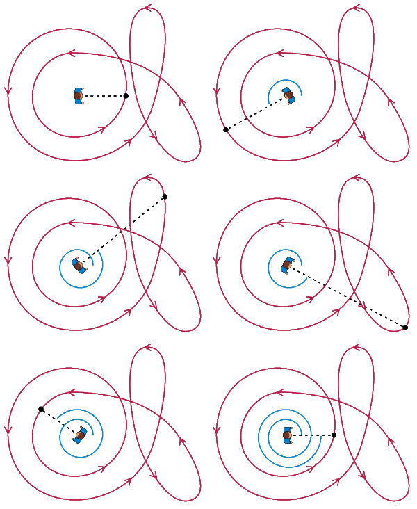
Por ejemplo, en la animación la acción es rotación (multiplicación por un complejo unitario) y la cantidad conservada es la norma del número complejo. En otras palabras, al ver las órbitas de la acción del grupo se obtienen las cantidades conservadas por dicha acción. Es importante el notar que las órbitas proveen una forma de visualizar el grupo que actúa sobre el espacio vectorial, por ejemplo en la anterior animación es posible ver que la forma del grupo que actúa es un circulo (complejos unitarios). Por esta razón es que el estudio de las acciones de grupos recibe el nombre de teoría de la representación, puesto que al ver las acción del grupo se ve indirectamente la forma del grupo en sí. 

La idea es que una acción de un grupo puede relacionarse con una acción local de su álgebra de Lie sobre el espacio tangente, o equivalentemente, la derivada de la acción puede verse como una especie de campo vectorial definido sobre el espacio vectorial. El espíritu del teorema de Noether es que, al igual que pasa en calculo multivariado, la integral cerrada sobre cualquier superficie de un campo conservativo siempre da 0, es decir se tiene una conservación del flujo del campo vectorial. 

Es posible pensar que la acción de un grupo produce de alguna manera un campo conservativo puesto que en la mayoría de los casos las acciones son bien portadas, es decir, son suaves. El problema con campos conservativos es que tienen singularidades, cosa que no pasa con una acción bien portada. 

Al ser el flujo conservado dentro de una superficie cerrada, esto da que la cantidad de masa dentro de la superficie es una cantidad conservada. 

Lo interesante es ver que cada vez que se tiene una acción sobre un espacio vectorial se pueden encontrar cantidades conservadas, aunque el encontrar dichas cantidades algunas veces es una tarea un poco difícil. 

Invariant polynomials and geometric transformations

A couple days ago, I stumbled over a really interesting problem looking for something to post for #ProblemOfToday. It was a problem that appeared in the 1989 Putman exam and reads as follows

"Prove that if 

$11z^{10}+10 i z^9 + 10 i z -11 =0$

then $|z|=1$."

It is a really nice problem in itself, but after thinking a bit on it, I thought what was so special about this specific coefficients to have this nice property. First, the polynomial can be analyzed in an even nicer way. By doing the transformation $z\mapsto i z$ we can see that the polynomial gets mapped (up to a negative sign) to:

$11z^{10}+10z^9+10z+11$

In this form one can see better how is the dependence of the polynomial on one of the coefficients (say 10), and can quickly ask a generalization of this particular problem:

If 

$(n+1)z^n+nz^{n-1}+n z+ (n+1)=0$

then $|z|=1$ for $n\in\mathbb{Z}/\{0\}$.

Doing a couple of special cases, one can get convinced that actually the previous statement holds true. 

$n=-4$ 

$n=10$

In the general case maybe the answer relies in a geometric argument. The polynomials $p_n(z)=(n+1)z^n+nz^{n-1}+n z+ (n+1)$ have the peculiarity that their roots are invariant under the  inversion of the complex plane, i.e. by doing the transformation $z \mapsto \frac{1}{z}$, we have that

$p_n(z)=z^np_n\left(\frac{1}{z}\right)$

that is, roots are mapped into roots by the inversion. 

Therefore, if there is a root bigger than 1, there should be a root smaller than 1 and vice-versa. It is not difficult to see that here cannot be a root bigger than 1, as $(n+1)z^n+nz^{n-1}$ and $n z+ (n+1)$ would have to be equal in modulus, but their orders of magnitude are different. 

Another way of proving this is by analyzing $p_n\left( e^{i \theta}\right)$. After a little simplification we have that $p_n\left( e^{i \theta}\right)=2e^{\frac{i \theta n}{2}}\left( n\cos\left( \frac{(n-2)\theta}{2}\right)+(n+1)\cos\left( \frac{n\theta}{2}\right)\right)$, which can be found to have exactly $n$ real roots for $\theta$. Hence all roots of $p_n$ lie on the unit circle.

The interesting fact is that for $n\to\pm\infty$, the roots of $p_n(z)$ become dense on $S^1$

For example, the graph of the absolute value of $p_21(z)$ is given by

where the $S^1$ can be seen. Likewise, for negative values of $n$ we can recover $S^1$

It looks like the $p_n(z)$ can be thought as some orthogonal polynomials whose support is $S^1$, and for the same reason, it is also natural to think that they can be eigenfunctions (up to a renormalization) of some operator (hopefully differential!).