A Generalization of Cauchy's Residue Theorem

In my research I use (or at least try to) some tools of complex analysis in order to evaluate infinite series arising from expressions involving the eigenvalues of an elliptic operator. The key ingredient is to use Cauchy's Residue Theorem (or equivalently Argument Principle) to rewrite a sum as a contour integral in the complex plane. 

Both incarnations basically state that it is possible to evaluate the closed integral of a meromorphic function just by looking at the residues that the contour encloses. 

If we have a function $f(z)$ holomorphic in a region $U\backslash\{z_0\}$ with a simple pole at $z=z_0$, then the integral 

$\int_\gamma f(z)dz$

fails to be zero just in its imaginary part. In some sense $f(z)$ provides a conservative field up to a phase. Namely, one can think of the pole inside $\gamma$ to be like a source of the field, and hence the failure of the integral to be zero. Since the integral only contributes with an imaginary part, it is possible to think that this constitutes something like a Berry phase, since it is proportional to the angle that the contour goes around the pole and the residue (charge) of it. 

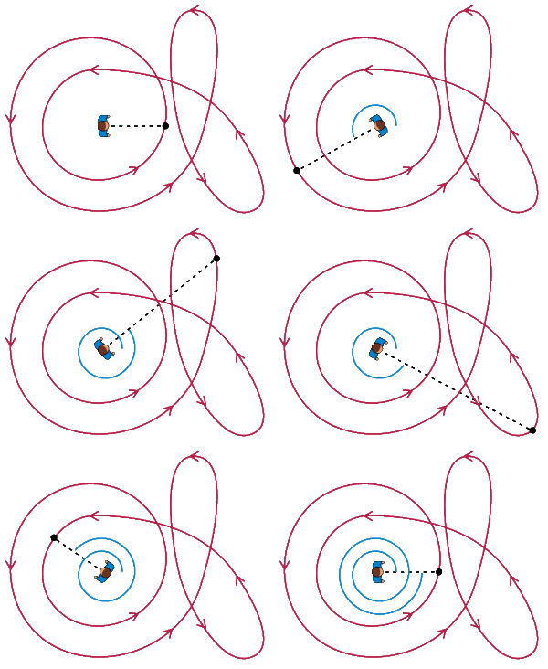
For instance, in the configuration on the left the contour makes an angle of $2\pi$ around the pole, while on the right it make only an angle of $\pi$ (if the contour is differentiable at the pole). If the pole lies on the contour, then the angle will be the difference of the angles made by the two tan gets at the point (the limit from the left and the right). In the case of a smooth contour, the only difference in both tangents is their direction, hence the angle of $\pi$.

If we denote by $\alpha(\gamma,z)$ the overall angle made by when we span the lines joining the point $z$ with points in $\gamma$, then we have a more general version of Cauchy's residue theorem

$\int_\gamma f(z)dz=\alpha(\gamma,z_0)\text{ Res }(f(z),z_0) i$

Note that for this result it is not needed for the contour $\gamma$ to be smooth, and it provides an extension of the usual residue theorem that uses the winding number. 

If the contour $\gamma$ is finite, it is customary to  understand for the inside of the contour to be the bounded pieces of the plane delimited by $\gamma$, but whenever we deal with infinite contour (e.g. a line) it is not so clear. 

In the first place, this result is valid only for bounded contours, so why bother with the infinite ones? If we  extrapolate this results to the Riemann sphere, dealing with infinite contours make sense, since they constitute great circles on the sphere. So in order to extend this to the Riemann sphere it is necessary to get rid of the ambiguity of what we understand for the inside of a contour. Or perhaps it is not. 

Following a little bit more the physical analogy for this result, one can also think that something like a conservation of charges might happen. In this case, the integral will give the same answer with any convention of inside only up to a sign difference. As the integral over a closed path in a region where the function is holomorphic is always zero, one could think of the total charge of the complex plane (or Riemann sphere) to be zero.

For this reason, it is usual to define the residue of a function at infinity to be such that the sum of all the residues of the function give zero, including the residue at infinity. Hence the negative sign in its definition

$\text{ Res }(f(z),\infty)=-\text{ Res }\left(\frac{1}{z^2}f\left(\frac{1}{z}\right),0\right)$

and the residue theorem for infinite contours (or equivalently for the Riemann sphere) reads

$\int_\gamma f(z)dz =i \sum_{\text{ poles }}\alpha(\gamma,w) \text{ Res }(f(z),w)$

where the poles $w$ can include residue at infinity.

Therefore expression like 

$\int_{-i\infty}^{i\infty} \frac{1}{z-1}dz$

can be evaluated using the residue theorem without any ambiguity on to which half plane to look for residues. As the function $f(z)=\frac{1}{z-1}$ has a residue at infinity of $-1$ and the contour $\gamma$ passes through infinity, this residue only contributes with $(\pi)(-1)$ to the integral. Choosing the convention of inside meaning to be to the left of the contour, it is just needed to analyze the left half plane. Thus this integral gives

$\int_{-i\infty}^{i\infty} \frac{1}{z-1}dz=-\pi i$

When grabbing the right half plane, we have to include the residue at $z=1$, but we have to change sign to the integral, hence it will give

$\int_{-i\infty}^{i\infty} \frac{1}{z-1}dz=-i\alpha(\gamma, 1)\text{ Res }(f(z),1)-i\alpha(\gamma, \infty)\text{ Res }(f(z),\infty)$

$=-2\pi i+\pi i=-\pi i$

Acciones y el Teorema de Noether

Este semestre estoy tomando una clase de teoría de invariantes. Básicamente la clase trata de estudiar los espacios invariantes resultantes de una acción de un grupo sobre un espacio vectorial y de analizar la descomposición de las órbitas en subespacios invariantes. Es un tema muy interesante y divertido de estudiar. 

Unos de los invariantes más famosos ocurren en el estudio del álgebra lineal. Que la traza y el determinante de una matriz permanecen igual bajo cambios de bases son resultados que provocan el deleite de chicos y grandes. Acá lo que se hace es que se estudia el espacio $M_n$ de las matrices $n\times n$, digamos, sobre el campo de números complejos, luego se ve la acción del grupo $U(n)$ sobre $M_n$ por medio de

$g.A\mapsto g^{-1} A g$

y se analizan los invariantes de la acción. 

Ya que $\det$ es un homomorfismo de anillos entre matrices y números complejos, tenemos que el determinante de una matriz es preservado por la acción:

$\det(A)=\det (g.A)$

y de acá podemos ver que el polinomio característico de $A$ es otro invariante de la acción. Con esto, los coeficientes del polinomio característico también son conservados por el cambio de base, y según las formulas de Vieta, dichos coeficientes son simplemente las funciones simétricas elementales de los valores propios de la matriz $A$, siendo el término constante el determinante de la matriz y el término de grado $n-1$ la traza de la matriz. 

Luego de analizar un poco esta situación, nos damos cuenta que la única información relevante de una matriz $A$  para esta acción son los valores propios de la misma. En cierto sentido esta es la información que se conserva al efectuar la acción. 

De una manera similar, al considerar la acción de $SL(n)$ sobre $M_n$ por 

$g.A\mapsto gA$

se tiene que la cantidad conservada por esta acción es $\det(A)$. 

Este fenómeno es un poco más conocido en el ámbito físico. Es muy sabido que dentro de un sistema, las simetrías corresponden con cantidades conservadas. Quizás esto sea un poco más familiar al ser referido por su nombre artístico, el Teorema de Noether. Muchos hemos visto la prueba de este teorema, la cual quizás es un bonito ejercicio de calculo multivariado, en donde se utiliza el concepto de simetría para encontrar que la el cambio de una cantidad del sistema es 0. 

Una simetría de un sistema no es más que un invariante proveniente de la acción de un grupo. 

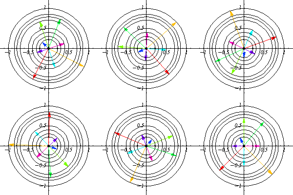
Por ejemplo, en la animación la acción es rotación (multiplicación por un complejo unitario) y la cantidad conservada es la norma del número complejo. En otras palabras, al ver las órbitas de la acción del grupo se obtienen las cantidades conservadas por dicha acción. Es importante el notar que las órbitas proveen una forma de visualizar el grupo que actúa sobre el espacio vectorial, por ejemplo en la anterior animación es posible ver que la forma del grupo que actúa es un circulo (complejos unitarios). Por esta razón es que el estudio de las acciones de grupos recibe el nombre de teoría de la representación, puesto que al ver las acción del grupo se ve indirectamente la forma del grupo en sí. 

La idea es que una acción de un grupo puede relacionarse con una acción local de su álgebra de Lie sobre el espacio tangente, o equivalentemente, la derivada de la acción puede verse como una especie de campo vectorial definido sobre el espacio vectorial. El espíritu del teorema de Noether es que, al igual que pasa en calculo multivariado, la integral cerrada sobre cualquier superficie de un campo conservativo siempre da 0, es decir se tiene una conservación del flujo del campo vectorial. 

Es posible pensar que la acción de un grupo produce de alguna manera un campo conservativo puesto que en la mayoría de los casos las acciones son bien portadas, es decir, son suaves. El problema con campos conservativos es que tienen singularidades, cosa que no pasa con una acción bien portada. 

Al ser el flujo conservado dentro de una superficie cerrada, esto da que la cantidad de masa dentro de la superficie es una cantidad conservada. 

Lo interesante es ver que cada vez que se tiene una acción sobre un espacio vectorial se pueden encontrar cantidades conservadas, aunque el encontrar dichas cantidades algunas veces es una tarea un poco difícil. 

Invariant polynomials and geometric transformations

A couple days ago, I stumbled over a really interesting problem looking for something to post for #ProblemOfToday. It was a problem that appeared in the 1989 Putman exam and reads as follows

"Prove that if 

$11z^{10}+10 i z^9 + 10 i z -11 =0$

then $|z|=1$."

It is a really nice problem in itself, but after thinking a bit on it, I thought what was so special about this specific coefficients to have this nice property. First, the polynomial can be analyzed in an even nicer way. By doing the transformation $z\mapsto i z$ we can see that the polynomial gets mapped (up to a negative sign) to:

$11z^{10}+10z^9+10z+11$

In this form one can see better how is the dependence of the polynomial on one of the coefficients (say 10), and can quickly ask a generalization of this particular problem:

If 

$(n+1)z^n+nz^{n-1}+n z+ (n+1)=0$

then $|z|=1$ for $n\in\mathbb{Z}/\{0\}$.

Doing a couple of special cases, one can get convinced that actually the previous statement holds true. 

$n=-4$ 

$n=10$

In the general case maybe the answer relies in a geometric argument. The polynomials $p_n(z)=(n+1)z^n+nz^{n-1}+n z+ (n+1)$ have the peculiarity that their roots are invariant under the  inversion of the complex plane, i.e. by doing the transformation $z \mapsto \frac{1}{z}$, we have that

$p_n(z)=z^np_n\left(\frac{1}{z}\right)$

that is, roots are mapped into roots by the inversion. 

Therefore, if there is a root bigger than 1, there should be a root smaller than 1 and vice-versa. It is not difficult to see that here cannot be a root bigger than 1, as $(n+1)z^n+nz^{n-1}$ and $n z+ (n+1)$ would have to be equal in modulus, but their orders of magnitude are different. 

Another way of proving this is by analyzing $p_n\left( e^{i \theta}\right)$. After a little simplification we have that $p_n\left( e^{i \theta}\right)=2e^{\frac{i \theta n}{2}}\left( n\cos\left( \frac{(n-2)\theta}{2}\right)+(n+1)\cos\left( \frac{n\theta}{2}\right)\right)$, which can be found to have exactly $n$ real roots for $\theta$. Hence all roots of $p_n$ lie on the unit circle.

The interesting fact is that for $n\to\pm\infty$, the roots of $p_n(z)$ become dense on $S^1$

For example, the graph of the absolute value of $p_21(z)$ is given by

where the $S^1$ can be seen. Likewise, for negative values of $n$ we can recover $S^1$

It looks like the $p_n(z)$ can be thought as some orthogonal polynomials whose support is $S^1$, and for the same reason, it is also natural to think that they can be eigenfunctions (up to a renormalization) of some operator (hopefully differential!).

Viernes 13

Como si no fuera poco con toda la propaganda sobre el fin del mundo, este 2012 comienza con otro indicio de mala suerte, hoy es viernes 13.

Tradicionalmente el viernes 13 ha sido catalogado como un día de mala suerte en muchas culturas del mundo, aunque posee una mayor influencia en la cultura anglosajona. En latinoamérica también es acostumbrado atribuirle malos augurios al martes 13, aunque ultimamente ha perdido seguidores quizás por la gran influencia cultural que el sistema anglo tiene sobre el resto del continente. También es curioso que en ambos casos la fecha es un número primo, aunque quizás tenga más relación con el hecho de que 13=12+1 (algo parecido pasa con el 6 y el 7).

Recuerdo que hace unos años atrás, en una clase de entrenamientos de olimpiadas surgió el tema del viernes 13. Estabamos recibiendo clase de probabilidades y nuestro profesor nos hizo el comentario acerca de que tan probable era en realidad que hubiera un viernes 13.

Si vemos tan solo la probabilidad de que el dia 13 de un mes sea viernes, estaríamos tentados a decir que dicha probabilidad es $1/7$, puesto que hay 7 posibles días de la semana (lunes, martes, etc.). Sin embargo el día de la semana y la fecha no son eventos completamente independientes, por lo tanto nuestro $1/7$ no es del todo correcto.

Para poder calcular la probabilidad correcta, es necesario contar cuantas veces un viernes 13 puede ocurrir. Para esto notamos que un mes tendrá un viernes 13 si dicho mes comienza en domingo. Este año 2012 habrán 3 viernes 13, en enero, en abril y en julio. Ahora, para poder calcular la probabilidad de un viernes 13 hay que tener claro lo que significa calcular la probabilidad. La forma más elemental de hacer esto es dividir el número de casos buscados sobre el número de casos totales, y para esto necesitamos saber que se entiende por casos totales en este contexto. Si el universo sobre el cual calculamos nuestra probabilidad es el número de viernes que hay en un año, tendríamos que nuestra probabilidad es $3/52$, ya que este año habrán 52 días viernes en total. Si por otro lado nuestro universo es el número de días 13, la probabilidad sería $3/12$, así que la pregunta central es ¿qué significa la probabilidad de un viernes 13? ¿Queremos calcular la probabilidad que un viernes sea 13? o ¿la probabilidad que un día 13 sea viernes? o ¿la probabilidad que un día sea viernes y sea 13? Creo que la ultima pregunta es la que describe mejor lo que andamos buscando, por lo tanto para el año 2012 tendríamos que la probabilidad es $3/366$.

El caso de 2012 es un caso especial, dado que es un año bisiesto, pero en general para calcular la probabilidad de que haya un viernes 13, es necesario analizar más detenidamente el calendario gregoriano. Al principio parecería suficiente ver dos casos, cuando el año es bisiesto y cuando no, sin embargo el calendario gregoriano es un poco más elaborado y un análisis un tanto más riguroso es necesario. 

Nuestro calendario tiene un período de 400 años, es decir, cada 400 años se repite exactamente el calendario, por ejemplo el 2412 comenzará en un domingo y habrán exactamente 3 viernes 13. Por lo tanto, contando el número de viernes 13 en un período de 400 años y dividiendo esto dentro del número total de días dará la probabilidad exacta de que haya un viernes 13.

Calculando este número (ya sea viendo un calendario, escribiendo un programa en excel o buscando en internet) da un total de 688 veces, así que dicha probabilidad es

$\frac{668}{149067}\sim 0.004481206437373798359127103919714$

Lo cuál es una probabilidad muy pequeña, sin embargo no es tan pequeña como para ser considerada de mala suerte. De hecho la mayoría de días 13 son viernes, por ejemplo, este año habrán 1 domingo, 2 lunes,

2 martes, 1 miércoles, 2 jueves, 3 viernes y 1 sábado que caerán días 13. Haciendo la misma cuenta sobre un período de 400 años es posible ver la distribución de días 13 en la semana. Tenemos que hay un total de 687 domingos, 685 lunes, 685, martes, 687 miércoles, 684 jueves, 688 viernes y 684 sábados que caen día 13, así que los viernes 13 son de hecho los días que más abundan, siendo los jueves 13 los menos frecuentes.

Sum of digits

Almost a month ago I participated in the Ibero-American College Olympiad thats was held in Quito  as team leader of the Guatemalan team. It had been almost 4 years now since I last participated in any olympiad-related event and sure enough, I was out of shape.  It is well known that mathematics is like any other activity, it requires constant practice and training, even more to make it in a competing level. 

I had a really good time remembering my Olympic times, but it also reminded my how out of shape I was. I must be that the type of mathematics used to do research is a bit different as the kind of skills that are used in competitions, as their goals are a bit different. None the less, this feeling made me start a personal goal: do at least one olympiad-type problem each day. With that in mind, I start this blog, were I post a problem everyday (first in my twitter and then I post the solution of the problem in the blog). Last week, when looking at one of the problems of the day, I noticed a very interesting pattern in the sum of the digits of the powers of 16.

I found the curious relation that the sum of the digits of $16^n$ is $6n+1$. This was something that I had never noticed before and I found it quite charming. After a bit, I started wondering if this sort of property was satisfied with some other powers, but found nothing like the powers of 16. It intrigued me then what was so special about 16 that made it have this beautiful property. 

Talking about this with my friend Esteban, I decided to seek for an easy proof of this fact that could unravel the mystery behind the 16, as no direct explanation seemed to appear.. What would the equivalent power be in a different base $b$ rather than 10?

Surprisingly enough, the core of this pretty property is hidden in the number 9. If you have a number $m$  which does not end in 1, $m$ and $m+9$ will have the same sum of digits. And what is the relation with 9 and 16? Well, $16^n$ always ends with 6, and when you multiply it by 16 we have that

 $16^{n+1}=16^n\cdot 10+16^n\cdot 6$. 

The first summand will have the same sum as $16^n$. Now the magic happens with the second summand. As it ends with 6, when performing the multiplications as we all learned in elementary school, the first operator that we make is $6\times 6=36=3\times 10+6$, thus the 30 adds up with the tenths of the first summand and voilà, there appears the 9. Then to compute the new number $(16^{n+1})$, we only have to keep performing this algorithm as in elementary school, and we end up having that the new number is going to have the same sum of digits as the one before, except by the digit of the units, which is 6. Therefore by induction we have that the sum is to have the desired form. 

By looking at this, we can easily find other numbers that work, for example the powers of $10^k+6$ will do the job. Here we can notice then that the special duty is made by the number 6, as $6^2=36$ whose sum of digits equals 9 and ends also in 6. So hence, when looking at different bases other than 10, we can find something similar happening. We need to have then a base $b$ and a digit $d$ such that:

• $d^2$ ends in $d$
• the sum of the digits of $d^2$ is equal to $b-1$.

In other words, we need to find pairs $(b,d)$ such that

$d^2=(b-1-d)b+d$

i.e.

$d^2+d(b-1)-b(b-1)=0$

which will have integer solutions iff 

$(b-1)^2+4b(b-1)=5b^2-6b+1=(5b-1)(b-1)$

is a perfect square. This is a diophantine equation of order two, which have integer solutions. For instance another solutions are $(65,40), (442, 273), (3026, 1870)$. One way of analyzing this equation can be by the method I described earlier.

Thus, similar properties are satisfied by $65^k+40$, $442^k+273$ and $3026^k+1870$ in base $65, 442$ and $3026$ respectively and $k>0$. It is a neat property and special also because it happens to be the case that we use a base that satisfy this diophantine equation. 

Reordenando Cifras

Hace unos días me reencontré con unos viejos amigos de matemática que no veía hacía un par de años, y regresando en el tráfico pensaba sobre un pequeño comentario que hicimos con Jóse Carlos al intercambiar números telefónicos.

Unos años atrás, Jóse Carlos poseía algo que todo matemático codicia: un número telefónico que es primo. Sin embargo ahora años después cuenta con otro número. Al darle mi número, le recordé que es primo, y al particionarlo en orden ascendente en pares y tríos, los números resultantes también son primos. Para mencionarme una propiedad interesante de su número, él me dijo que al realizar una permutación de este y ordenarlo a pares se obtenían que los cuatro números obtenidos eran múltiplos dos a dos.

Pensando en propiedades de números que surgían al ser reordenados, una pregunta natural es

¿de cuántas maneras se pueden reordenar las cifras de un número para obtener números distintos?

Para un número en particular, esta pregunta es fácil de calcular, por ejemplo si vemos el número 122 podemos ver que solamente se pueden reordenar sus cifras de 3 formas diferentes

122

212

221

o para el número 524, se tienen 6 formas diferentes

245

254

425

452

524

542

Sin embargo, si llamamos

$\nu(n)=$número de números distintos obtenidos al permutar las cifras de $n$

una expresión general de $\nu(n)$ resulta muy complicada de escribir, si no es que imposible, puesto que la aparición de dígitos en la expansión decimal de $n$ no es algo fácil de controlar.

Por ejemplo se tiene que la función no es monótona y alcanza valores bajos infinitamente, e.g. $\nu(11\dots 1)=1$ para cualquier cantidad de 1´s.

Como es cosa usual con funciones número-teoréticas, un segundo paso después de buscar expresiones exactas, es buscar comportamientos asintóticos.

Una forma de encontrar esta aproximación es por medio de hallar una expresión semi-explícita para $\nu(n)$.

Sea $n_i$ es número de dígitos $i$ que aparecen en la representación decimal de $n$ y $N$ el número de dígitos de $n$. Entonces

$\nu(n)=\binom{N}{n_0}\binom{N-n_0}{n_1}\binom{N-n_0-n_1}{n_2}\dots \binom{N-n_0-n_1-\dots -n_8}{n_9}$

$=\binom{N}{n_0\, n_1\, n_2\, \dots\, n_9}$

donde el término anterior es el coeficiente multinomial del número de dígitos.

Para calcular una expresión asintótica, podemos decir que para valores grandes de $n$ genéricamente se tiene que $n$ posee sus dígitos uniformemente distribuidos, por lo tanto

$N\sim \log n$

y

$n_i\sim \frac{N}{10}=\frac{\log n}{10}$

por lo tanto tenemos que $\nu(n)$ se comporta como

$\nu(n)\sim \binom{\lfloor\log n\rfloor}{\left\lfloor\frac{\log n}{10}\right\rfloor\, \left\lfloor\frac{\log n}{10}\right\rfloor\,\dots \, \left\lfloor\frac{\log n}{10}\right\rfloor}$

$=\frac{\lfloor\log n\rfloor!}{\left[\left\lfloor\frac{\log n}{10}\right\rfloor!\right]^{10}}$

Aca está la gráfica de la asíntota para $n\leq 100000$

y como se puede ver, asíntoticamente la función crece muy rápido, por lo que para valores grandes de $n$, es posible reordenar sus cifras y encontrar números con propiedades interesantes relacionadas con $n$ dada la gran cantidad de opciones disponibles.

Hearing the string, not the shape

Last week I went to a very interesting summer school about algebraic and topological methods in quantum mechanics. It was a very eclectic crowd between mathematicians and physicists and undergrads, grads, postdocs and professors.

There were lectures, talks and something really interesting called short communications. The idea of these was to encourage participants to present some interesting facts that came from the main lectures. In one of these communications, a group presented the famous topic about hearing the shape of a drum, and their presentation made me think about the mathematical formulation of what does it mean to hear a a sound, and moreover why do we hear certain type of sound and not another.

Suppose we are listening to a string sound, like a guitar. The most basic model of this is the wave equation

$\partial_{tt}\psi=\Delta \psi$

subject to the initial conditions $\psi(0,x)=f(x)$ and $\partial_t \psi(0,x)=g(x)$.

Solving this equation models the behavior of the vibrating string. This PDE can be solved using separation of variables and fourier analysis for the initial conditions, and by these means, the associated wave frequency, can be thought as the separation constant, i.e. when supposing a solution of the form $\psi(t,x)=T(t)X(x)$, the above equation takes the form

$\frac{T''(t)}{T(t)}=\frac{X''(x)}{X(x)}$

Since the RHS is a function of $t$ and the LHS is a function of $x$, the only possible case is that they are equal to a constant (the separation constant) $\lambda$. When applying the initial conditions, the equation in $x$ is easier to solve,as it takes the form of an eigenvalue problem

$X''(x)=\lambda X(x)$

with $X(0)=0$. Notice that this equation does not have a time dependence anymore, and the $\lambda$ parameter is what at the end determines the frequency (frequencies) at which the string resonates. Moreover, the initial position $f(x)$ and initial velocity $g(x)$ do not play a role with the solution of this part of the wave equation, and hence, do not affect with the value of the frequencies $\lambda$. This is the main reason why it really doesn't matter how hard or where to pinch a guitar string, it will always sound the same, maybe a little louder or softer, but the same type of sound. An E string will always sound E, no matter where or how you pinch it.

This means that the sound is an intrinsic characteristic of a material, is not really dependent on the force applied to it but to its shape and physical characteristics.